
Gradient
Derivatives
- We can also interpret the slope as:
- If I nudge x, how does y change?

Pretend that multivariable funciton is univariate, then take derivative as normal. This is a partial derivative.
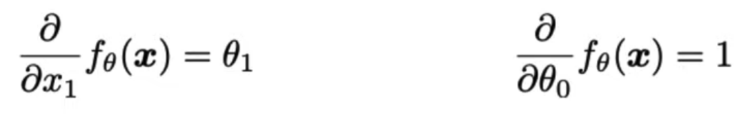
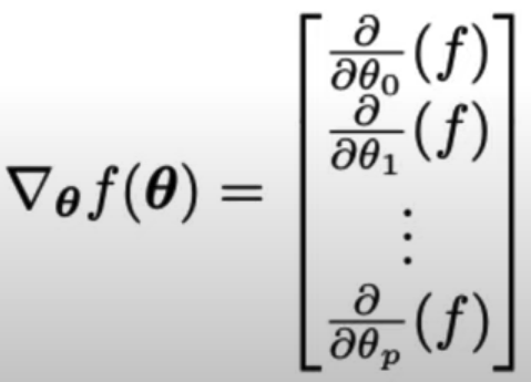
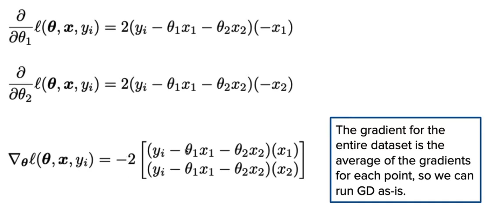
- The gradient extends the derivative to multiple variables.
- Vector-valued function (always outputs a vector).
- The gradient of f(θ) w.r.t. θ is a vector. Each element is the partial derivative for component of θ.
Using the Gradient
Gradient w.r.t. θ encodes where θ should "move".
- Left: θ should move in the positive direction
- Right: θ should move in negative direction
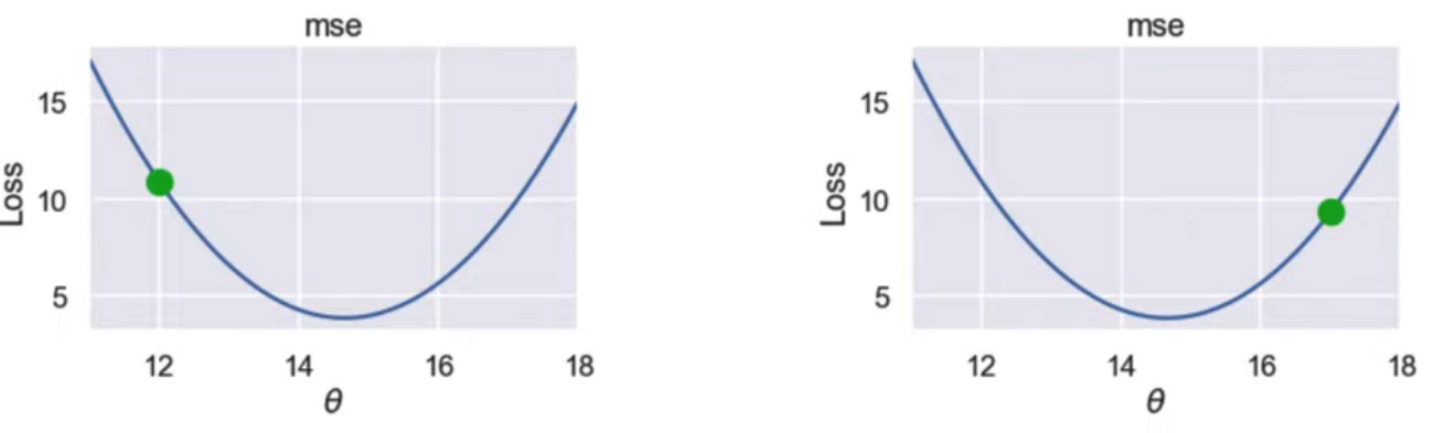
- Left plot: gradient - , want θ +
- Right plt: graident +, want θ -
- Idea: Move θ in negative direction of gradient.
Gradient descent algorithm: nudge θ in negative gradient direction until θ converges.
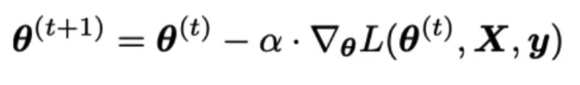
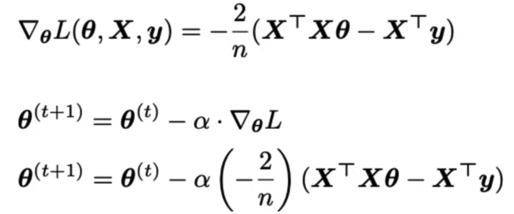
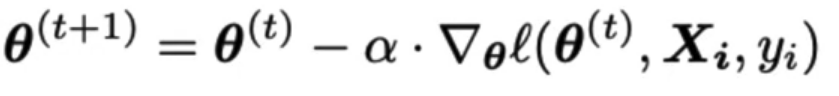
Batch gradient descent update rule:
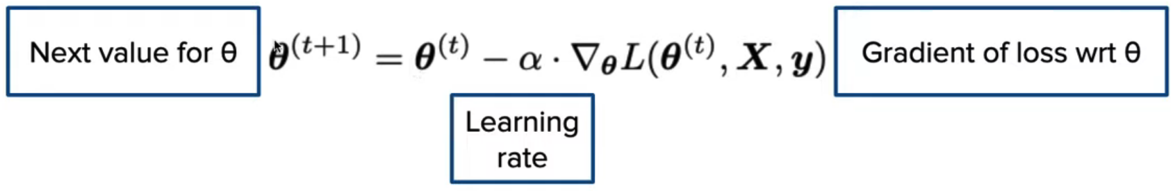
θ: Model weights
L: loss function
α: Learning rate, usually samll constant
y: Ture values from training data
Update model weights using update rule:
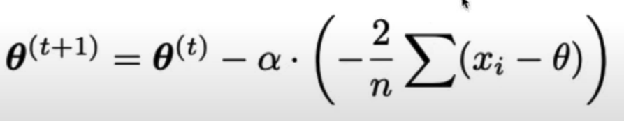
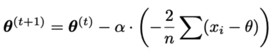
Gradient Descent for MSE
- For constant model using MSE loss, we have:

So the update rule is:
The Learning Rate
- α called the learning rate of gradient descent.
- Higher values can converge faster since θ changes more each iteration.
- But α too high might cause GD to never converge!
- α too low makes GD take many iterations to converge.
Question:
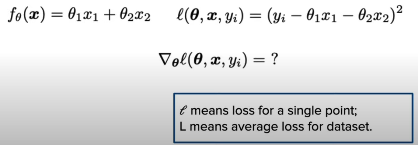
Answer:
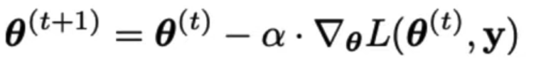
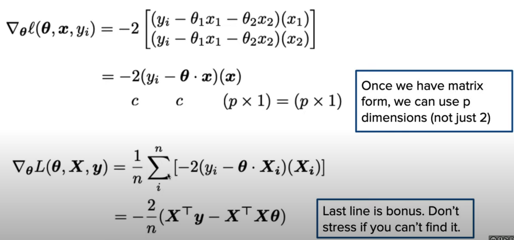
In Matrix Form:
Update Rule:
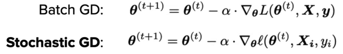
Stochastic Gradient Descent (SGD)
- Can perform update using one data point instead of all the data points.
SGD usually converges faster than BGD in practice!
SGD Algorighm
- Initialize model weights to zero
- Shuffle input data.
- For each point in the shuffled input data, perform update:
- Repeat steps 2 and 3 until convergence.
Each individual update is called an iteration.
Each full pass through the data is called an epoch.
Example:
- BGD update rule for constant model, MSE loss:
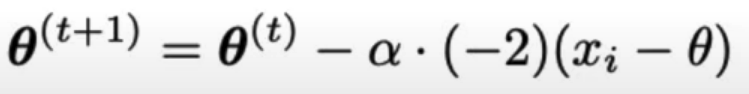
- SGD update rule for constant model, MSE loss:
Why does SGD perform well?
Intuition: SGD "does more" with each data point.
- E.g. Sample of size 1 million
- BGD requires ≥1 million calculations for one update
- SGD will have updated weights 1 million times!
- However:
- BGD will always move towards optima
- SGD will sometimes move away because it only considers one point at a time.
- SGD still does generally better in spite of this.
Convexity
For a convex funtion f, any local mimnimum is also a global minimum.
- If loss function convex, gradient descent will always find the globally optimal minimizer.
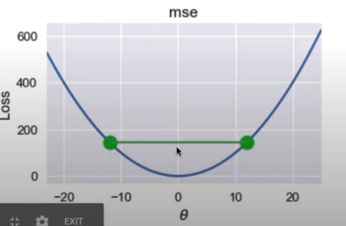
Formally, f is convex if:
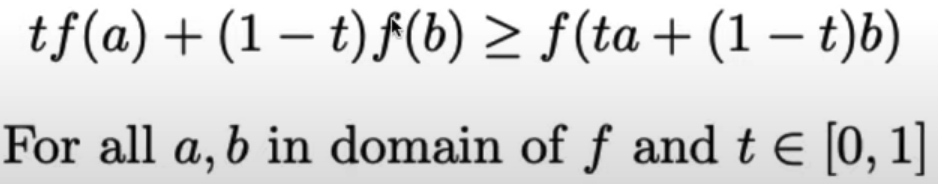
- RTA: If I draw a line between two points on curve, all values on curve need to be on or below line.
- MSE loss in convex:
Huber Loss
- What if we want the outlier-robust properties of MAE?
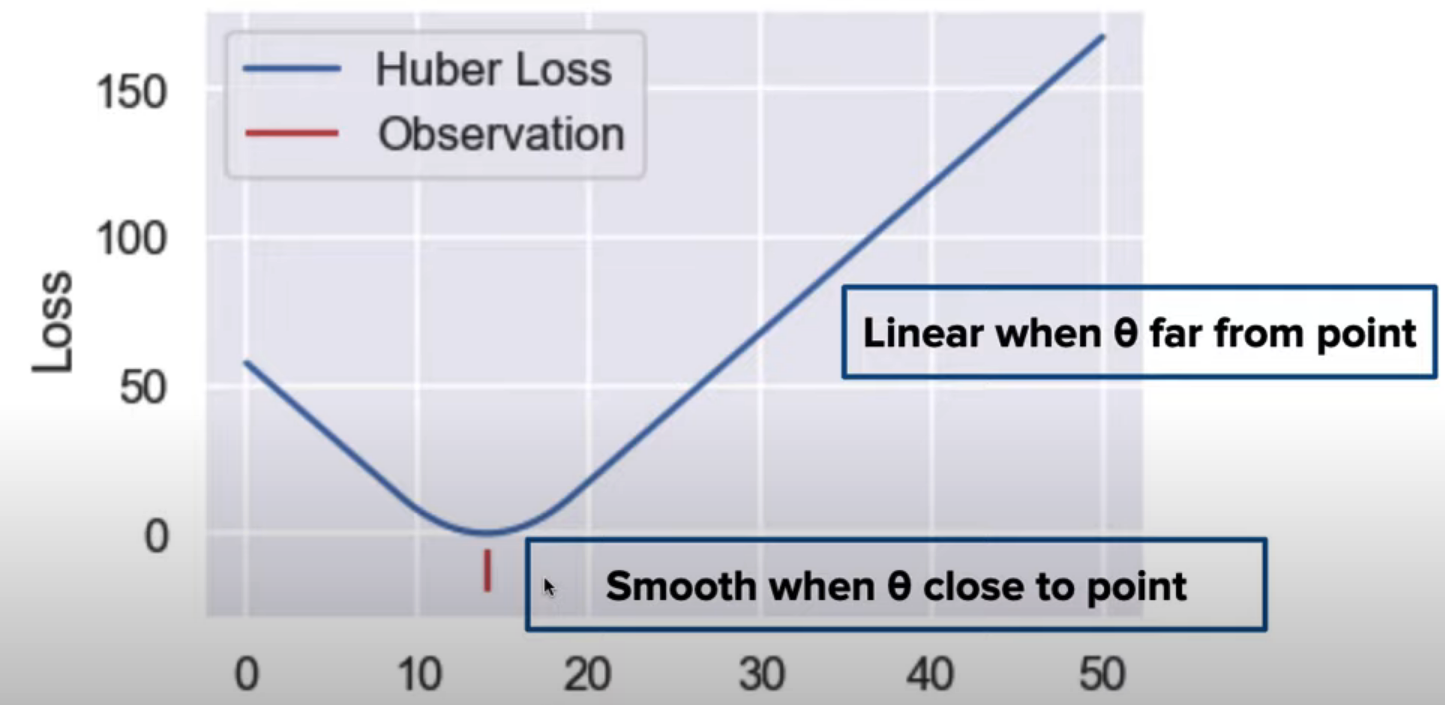
- Use Huber Loss:
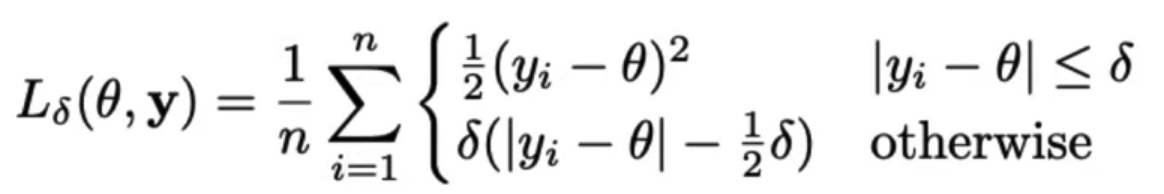
- Behaves like MAE loss when points far from θ
- But like MSE loss when points close to θ
- ∂ is a parameter that determines where Huber loss transitions from MSE to MAE.
- No analytic solution (unlike MSE and MAE)
- But differentiable everywhere, so we can use GD!
- Try taking the derivative and running GD for practice.
'Computer Science 🌋 > Machine Learning🐼' 카테고리의 다른 글
| Foundation of Machine Learning (0) | 2023.05.31 |
|---|---|
| SQL in Pandas Review (0) | 2023.05.30 |
| Text Fields Review (0) | 2023.05.30 |
| EDA Review (0) | 2023.05.30 |
| Data Cleaning Review (0) | 2023.05.28 |
Gradient
Derivatives
- We can also interpret the slope as:
- If I nudge x, how does y change?
Pretend that multivariable funciton is univariate, then take derivative as normal. This is a partial derivative.
- The gradient extends the derivative to multiple variables.
- Vector-valued function (always outputs a vector).
- The gradient of f(θ) w.r.t. θ is a vector. Each element is the partial derivative for component of θ.
Using the Gradient
Gradient w.r.t. θ encodes where θ should "move".
- Left: θ should move in the positive direction
- Right: θ should move in negative direction
- Left plot: gradient - , want θ +
- Right plt: graident +, want θ -
- Idea: Move θ in negative direction of gradient.
Gradient descent algorithm: nudge θ in negative gradient direction until θ converges.
Batch gradient descent update rule:
θ: Model weights
L: loss function
α: Learning rate, usually samll constant
y: Ture values from training data
Update model weights using update rule:
Gradient Descent for MSE
- For constant model using MSE loss, we have:
So the update rule is:
The Learning Rate
- α called the learning rate of gradient descent.
- Higher values can converge faster since θ changes more each iteration.
- But α too high might cause GD to never converge!
- α too low makes GD take many iterations to converge.
Question:
Answer:
In Matrix Form:
Update Rule:
Stochastic Gradient Descent (SGD)
- Can perform update using one data point instead of all the data points.
SGD usually converges faster than BGD in practice!
SGD Algorighm
- Initialize model weights to zero
- Shuffle input data.
- For each point in the shuffled input data, perform update:
- Repeat steps 2 and 3 until convergence.
Each individual update is called an iteration.
Each full pass through the data is called an epoch.
Example:
- BGD update rule for constant model, MSE loss:
- SGD update rule for constant model, MSE loss:
Why does SGD perform well?
Intuition: SGD "does more" with each data point.
- E.g. Sample of size 1 million
- BGD requires ≥1 million calculations for one update
- SGD will have updated weights 1 million times!
- However:
- BGD will always move towards optima
- SGD will sometimes move away because it only considers one point at a time.
- SGD still does generally better in spite of this.
Convexity
For a convex funtion f, any local mimnimum is also a global minimum.
- If loss function convex, gradient descent will always find the globally optimal minimizer.
Formally, f is convex if:
- RTA: If I draw a line between two points on curve, all values on curve need to be on or below line.
- MSE loss in convex:
Huber Loss
- What if we want the outlier-robust properties of MAE?
- Use Huber Loss:
- Behaves like MAE loss when points far from θ
- But like MSE loss when points close to θ
- ∂ is a parameter that determines where Huber loss transitions from MSE to MAE.
- No analytic solution (unlike MSE and MAE)
- But differentiable everywhere, so we can use GD!
- Try taking the derivative and running GD for practice.
'Computer Science 🌋 > Machine Learning🐼' 카테고리의 다른 글
| Foundation of Machine Learning (0) | 2023.05.31 |
|---|---|
| SQL in Pandas Review (0) | 2023.05.30 |
| Text Fields Review (0) | 2023.05.30 |
| EDA Review (0) | 2023.05.30 |
| Data Cleaning Review (0) | 2023.05.28 |